Dominican Inflation Data • databcrd

library(databcrd)
library(ggplot2)
library(dplyr)

Inflation is undoubtedly one of the most important macroeconomic variables and the core of the monetary policy in the Dominican Republic. Its evolution affects the stability of real variables such as consumption and investment, attracting analysts’ attention and being frequently consulted.

This article demonstrates how to quickly access inflation expectations in the Dominican Republic using the databcrd package, specifically the get_ipc_data() function.

Published Inflation Breakdowns

General: National inflation without breakdowns
By groups: Breakdown by groups of goods and services
By regions: Inflation specific to the country’s macro-regions
By components: Inflation of tradable and non-tradable goods
Core: Core inflation, excluding volatile items
Items:

With the package, all inflation breakdowns can be accessed using the get_ipc_data() function. Simply specify the desagregacion argument. The possible values are: "general", "grupos", "subyacente", "regiones", "tnt", and "articulos".

General Inflation

With get_ipc_data("general"), the updated general inflation data is downloaded, including the index (ipc), monthly variation (ipc_vm), year-over-year variation (ipc_vi), variation since December (ipc_vd), and the 12-month average variation (ipc_p12).

inflacion_general <- get_ipc_data("general")
inflacion_general
#> # A tibble: 494 × 8
#>    fecha      year    mes   ipc ipc_vm ipc_vd ipc_vi ipc_p12
#>    <date>     <chr> <dbl> <dbl>  <dbl>  <dbl>  <dbl>   <dbl>
#>  1 1984-01-01 1984      1  1.38  1.74    1.74   7.05    5.57
#>  2 1984-02-01 1984      2  1.42  2.81    4.60  11.2     6.01
#>  3 1984-03-01 1984      3  1.44  1.23    5.89  11.9     6.52
#>  4 1984-04-01 1984      4  1.46  1.57    7.55  14.9     7.36
#>  5 1984-05-01 1984      5  1.48  1.20    8.84  15.2     8.26
#>  6 1984-06-01 1984      6  1.54  4.31   13.5   19.6     9.49
#>  7 1984-07-01 1984      7  1.56  1.29   15.0   20.7    10.8 
#>  8 1984-08-01 1984      8  1.57  0.455  15.5   20.1    12.0 
#>  9 1984-09-01 1984      9  1.64  4.69   20.9   24.8    13.7 
#> 10 1984-10-01 1984     10  1.68  2.34   23.8   26.3    15.4 
#> # ℹ 484 more rows

Let’s generate graphs for each variable.

# Function to plot inflation data
plot_ipc_data <- function(data, variable, title, start_year = 2018) {
  data |>
    filter(year == start_year) |> 
    ggplot(aes(x = fecha, y = {{ variable }})) +
    geom_line() +
    theme_minimal() +
    ggtitle(title) +
    theme(
      axis.title = element_blank(),
      plot.title.position = "plot"
    )
}

plot_ipc_data(inflacion_general, ipc, "Consumer Price Index")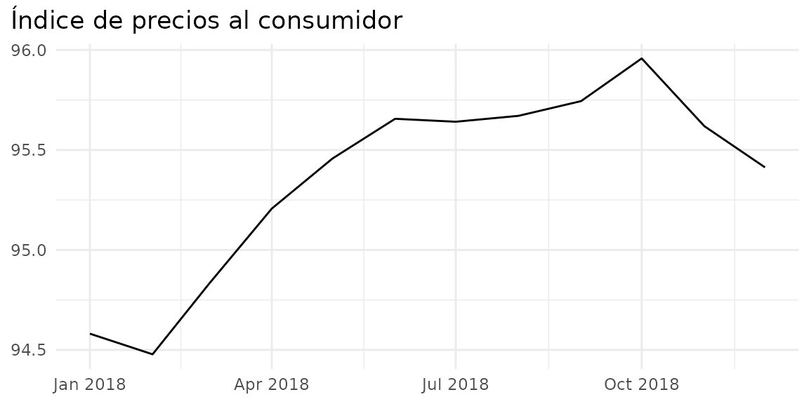

plot_ipc_data(inflacion_general, ipc_vm, "Monthly Variation of CPI") +
  scale_y_continuous(labels = \(x) scales::comma(x, accuracy = 0.1, suffix = "%"))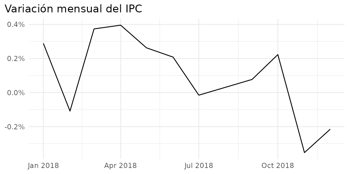

plot_ipc_data(inflacion_general, ipc_vi, "Year-over-Year Variation of CPI") +
  scale_y_continuous(labels = \(x) scales::comma(x, accuracy = 0.1, suffix = "%"))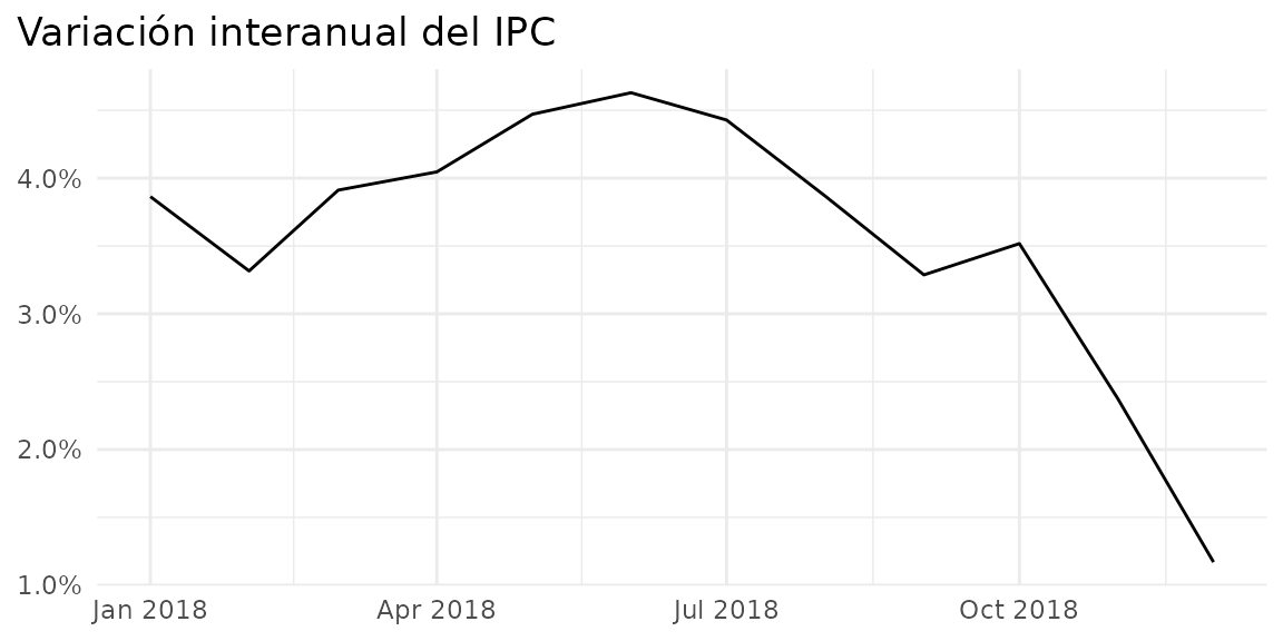

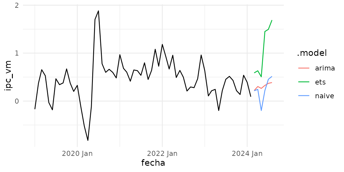
Now a naive forecast of inflation

library(tsibble)
#> Registered S3 method overwritten by 'tsibble':
#>   method               from 
#>   as_tibble.grouped_df dplyr
#> 
#> Attaching package: 'tsibble'
#> The following objects are masked from 'package:base':
#> 
#>     intersect, setdiff, union
library(fable)
#> Loading required package: fabletools
library(feasts)

ts_ipc <- inflacion_general |>
  mutate(fecha = yearmonth(fecha)) |>
  select(-mes) |>
  as_tsibble(index = fecha)

models <- ts_ipc |>
  model(
    ets   = ETS(box_cox(ipc_vm, 0.3)),
    arima = ARIMA(ipc_vm),
    naive = SNAIVE(ipc_vm)
  )

models
#> # A mable: 1 x 3
#>            ets                     arima    naive
#>        <model>                   <model>  <model>
#> 1 <ETS(A,N,A)> <ARIMA(3,1,1)(2,0,0)[12]> <SNAIVE>

models |>
  forecast(h = "6 months") %>% 
  autoplot(filter(ts_ipc, year > 2018), level = NULL) +
  theme_minimal()